Finding shortest paths and simulating black holes
What’s the shortest path between two points - A and B? Most people instinctively say it’s a straight line between those two points. Which is true on a flat 2D plane, but what about on the surface of the earth? What’s the shortest path between two points on the surface of the earth? Let’s ask Google:
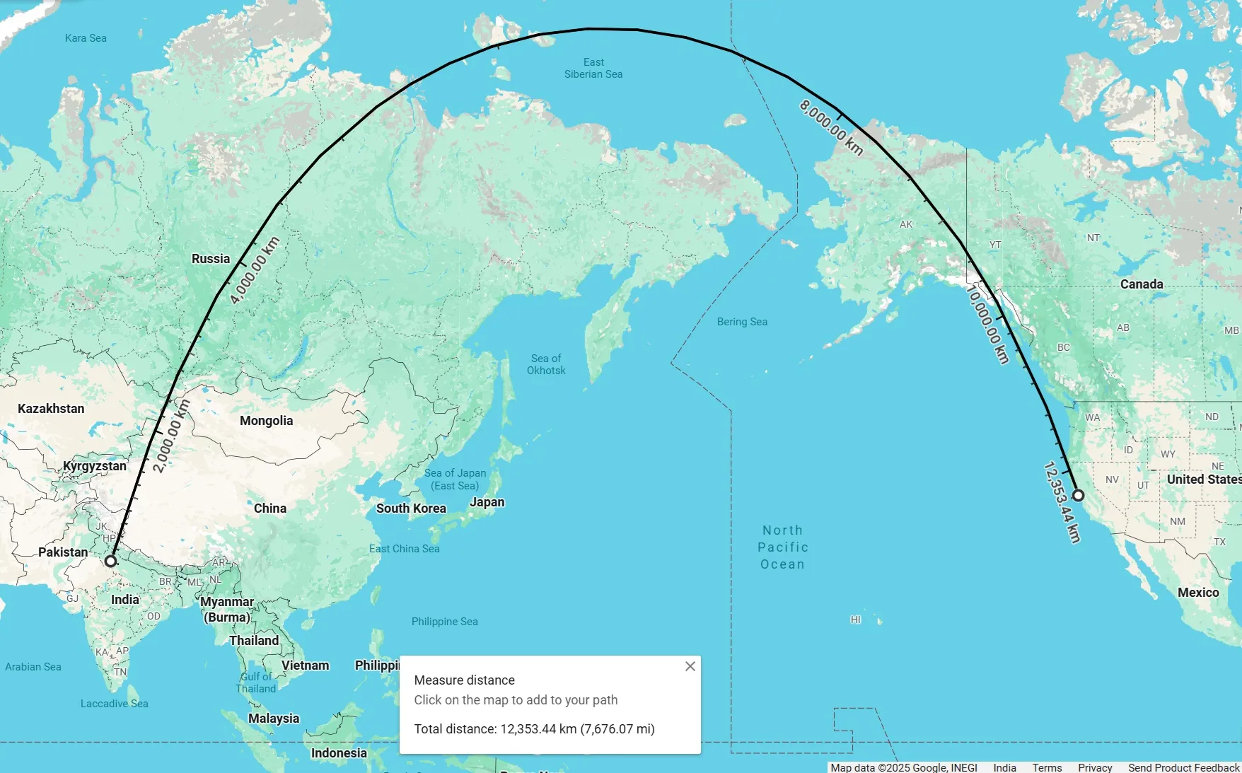
Shortest path between New Delhi and San Franciso on the map. © Google Maps.
That’s clearly not a straight line. So is Google Maps bugged, or is math bugged? Have we uncovered a conspiracy by Big Globe? Actually, turns out it is a straight line! But it’s a straight line on a sphere, and straight lines on a sphere aren’t straight on a 2D projection of the sphere, which is what a map is!

Shortest path between New Delhi and San Franciso on the globe. © Google Maps.
In fact, the most common projection used in maps, the Mercator Projection, infamously distorts distances. This results in countries farther from the equator appearing grossly distorted (made MUCH larger).
Distortions produced by the Mercator Projection: Jakub Nowosad, CC BY-SA 4.0, via Wikimedia Commons
So what gives? Can we generalize a way to always find the shortest path between two points, regardless of the surface we are working with? Turns out, yes, we can (more on this later)! This is known as Geodesics. If you have seen any videos about General Relativity on YouTube, you definitely have heard “Geodesic” at least once. In this blog, I will motivate why we need geodesics, and personally why I needed geodesics.
This blog contains math and code, but you can go through and understand the whole thing without actually doing either. You have to just trust me bro.

However, true satisfaction will only come when you actually do at least some of both, and see that it all works out. So, I will try to explain the math as well, but I will not go into too much detail. If you want to see the proofs, many good videos on YouTube explain them in detail. For the code, I will provide snippets, and a lengthier post about my path tracer will be coming soon.
Motivation
I must confess, I am not a mathematician. I am a Software Engineer. Normally, if for some reason I came across the math for geodesics, I would simply close that browser tab and move on. However, I was finally tackling a bucket-list hobby project I wanted to make for a long, long time. Unfortunately, skill and time issues were holding me back. The goal was to recreate the famous Interstellar scene of the black hole.
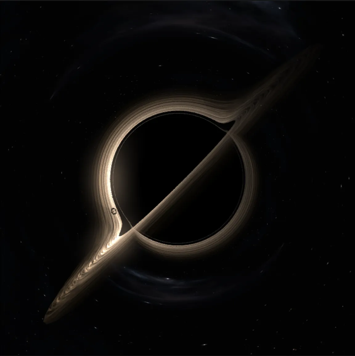
Image produced by my path tracer of a non-rotating black hole with an accretion disk.
This is the result. If this is not motivation enough, I really don’t know what is. Anyway, now that we know the payoff, time for the math (and code)!
Before I piss off the physicists and mathematicians
In order to keep this blog somewhat reasonable, I will be glossing over the whys and only focussing on the hows. My motivation, really, is to get that pretty image of the black hole. Maybe in the future, when my ChatGPT-Chromium-VSCode wrapper finally takes off and I make a gazillion dollars and retire, I will learn and write about the mysteries of the universe in more detail. Anyway, enjoy the ride!
The Plan
The plan is to learn:
- What’s a tensor?
- What the **** is a ?
- What’s a metric?
- The generalized distance formula
- The Bridge: The Euler-Lagrange Equation
- The Geodesic Equation
- Christoffel symbols
- A concrete example
When learning hard things, I find it helps to turn off your ape brain screaming “THIS IS TOO HARD! I DON’T UNDERSTAND! TURN AWAY NOW!”, and just follow the instructions. Often, once you go through the process once, it becomes clear that, in fact, it’s really easy, just bogged down by notation and tedium. If you are a programmer, this will probably be very easy for you. Really, you can understand the whole thing using high school calculus. Yeah you won’t be able to derive it but you can appreciate how it works, and that’s enough to get a pretty picture, so it’s good enough for me (for now).
What’s a tensor?
Let’s consult Wikipedia:
In mathematics, a tensor is an algebraic object that describes a multilinear relationship between sets of algebraic objects associated with a vector space. Tensors may map between different objects such as vectors, scalars, and even other tensors. There are many types of tensors, including scalars and vectors (which are the simplest tensors), dual vectors, multilinear maps between vector spaces, and even some operations such as the dot product. Tensors are defined independent of any basis, although they are often referred to by their components in a basis related to a particular coordinate system; those components form an array, which can be thought of as a high-dimensional matrix.
Yikes! Let me use programmer-translate on that: For our purposes, a tensor is simply a multi-dimensional array. You can define a tensor:
And it’s really just a 2D array like [[1, 0], [0, 1]]. But hold on a second…
What the **** is a ?
says “you need two indices and , to get a scalar value from this tensor.” Yes, and are just array indices! Okay, so.. how do we index them? You can simply index them like in your favorite language, but by convention, the indices start at 1 🤢 sorry. So, the components of the tensor can be accessed like
So, really, is sort of like saying g[i][j] = [[1, 0], [0, 1]].
Now, so far, and have been generic indices. You can get a value, say , but it doesn’t really mean anything. To be useful, we attach a coordinate system with a tensor! Let’s say we’re working on the 2D cartesian plane, so our coordinates are (The order is important!) This means, our first index, corresponds to the coordinate, and the second index, corresponds to the coordinate. Here’s all the components of the tensor above:
Here, corresponds to “how much of the component relates to the component”? This probably doesn’t make sense, so I introduce…
What’s a metric?
A metric, (a.k.a. a metric tensor, the “tensor” part is often omitted to make it sound mysterious and hard), is just a tensor that helps us calculate the distance between two points in a given space and coordinate system. I copied this from Wolfram, so it must be correct. So what does it look like? Well, you’ve already seen one! The tensor I’ve been using is a metric tensor for the flat 2D plane in cartesian coordinates !
Now, we can answer the question from the previous section, “how much of the component relates to the component”? Let’s take . This tells us, “how much of the direction relates to the ” direction? They’re the same, so the value is . Now, what about ? This tells us “how much of the direction relates to the direction?” These two directions are orthogonal (perpendicular), so the value is . Similarly, is , and is . Basically, moving in the direction doesn’t change your coordinate, and vice-versa.
Let’s see some other metric tensors, say for spherical metric tensor in spherical coordinates ( ):
And the Schwarzschild metric tensor in spherical coordinates ( ):
As an aside, this is the metric tensor that describes the space around a uncharged non-rotating black hole! This is the one used to create the image you saw above, although the one in Interstellar is a rotating black hole, which is described by the even more complicated Kerr Metric. However, you can’t really tell the difference. We’ll come back to this metric soon.
In any case, the metric tensor directly tells us how to calculate the distance between two points regardless of how complicated the underlying space is, as long as we are willing to put up with the tedious math. To do it we just have to integrate…
The generalized distance formula
Let me just hit you with the thing:
Let’s unpack this…
- is the metric tensor of the space you are working with
- is a compact way to refer to any of the coordinates in our system. It means whatever coordinate index you are using in place of , replace with that. So in our 2D system with coordinates , would be , and would be . This will make more sense momentarily.
- What the ?! Remember, , are just placeholders. You have to replace them with all the possible combinations of your coordinate system. The says after you do that, you sum them all together.
Fun aside: Physicists are lazy, and got tired of writing over and over again. So we just don’t write the , and anytime we have a repeated index like or , assume it is summed over all possible values for those indices. This has unfortunately caught on, much to the detriment to everyone learning this for the first time, and now it’s called “Einstein notation”. If you look online, you’ll see the distance formula written as . They are the same thing!
Let’s take our good old flat 2D plane with cartesian coordinates, . This means and have to take on the coordinates and . And we know the metric tensor for this space and coordinate system is
So, the distance formula in this space and coordinate system is:
We already know how to index the metric tensor, so we find the values like this: . And for the confusing part, and ! We just replace the whole thing by the coordinate, it not an exponent!
Plugging everything in to the equation, we get:
Does this look familiar? It should, because it’s just the Pythagorean theorem! This is saying, if we move some infinitesimal distance in the direction, and in the direction, the square of the total distance is the sum of squares of the individual distances! That wasn’t so hard, was it? Just a lot of symbols!
Well, that was pretty cool! However, we are still only getting the distance, not the path! To do that, we’ll need…
The Bridge: The Euler-Lagrange Equation
We have the equation for smallest distance, but what’s the shortest path corresponding to that distance? This is where the Euler-Lagrange equation comes in. This equation comes from the Calculus of Variations, and is really really cool! I won’t go into the details here, but you can watch this video to get a sense of what’s going on. All you need to know, the Euler-Lagrange equation is a way to find the function that minimizes (or maximizes) some quantity. In our case, we want to minimize the distance between two points. The Euler-Lagrange equation looks like this:
In our case, we want to minimize the distance, so we set . Now, is again a placeholder, so we have to replace it with a coordinate. And, means , the derivative of the coordinate with respect to the distance. This is just a fancy way of saying “the rate of change of the coordinate as we move along the path”. So, we have:
If you put your faith in me (and the many videos online), you can plug this into the Euler-Lagrange equation, and after a lot of algebra, you will get…
The Geodesic Equation
Ignoring all the indices and the , the bottom line is, if we are able to somehow solve this thing, it will give us the equations for the shortest path. However, notice the . Here, again, is a placeholder, and we have to replace it with a coordinate. Then, if we solve the equation, we will get another equation for the shortest path in that coordinate direction!.
Awesome! Now, what about the ? Well…
The Christoffel symbols
The Christoffel symbols are just functions of the metric. They are easily calculatable. But there is a slight problem. See if you can guess it.
Yes, pretty gnarly. Let’s unwrap this.
- and are also placeholders. You need to replace them with coordinates.
- The . The metric tensor is always a 2D matrix. So, you can calculate the inverse of that matrix. I’m going to use the notation (don’t @ me mathematicians). Note that this will also be a matrix of the same size. In fact, this is also a tensor, the inverse metric tensor! We define .
- We simply define .
Now notice, nothing here is super advanced stuff, just some linear algebra and partial derivatives. Pretty doable, we did this in high school! But the problem, as I’m sure you’ve noticed by now, is that the Christoffel symbols have indices. And, to calculate one symbol, we need indices. That’s a ridiculous amount of pure computation. Luckily, we don’t have to do it for our original use case, they’ve already been calculated, and we can just plug in the values, but if you are feeling particularly masochistic, do give it a try! If we have coordinates, there will be Christoffel symbols! Good luck!
Let me give you a Python snippet with a magic calculate_partial_derivative function to illustrate the point.
g = [[1, 0], [0, 1]]  # Some metric tensor
inv_g = [[1, 0], [0, 1]] # The inverse metric
coords = ['x', 'y'] # The coordinate axes

# We'll store the values like christoffel_symbols[f'{alpha}_{mu}_{nu}'] = value
christoffel_symbols = dict()

for alpha in coords:
for mu in coords:
for nu in coords:
 value = 0.0
 symbol = f'{alpha}_{mu}_{nu}'
 alpha_idx = coords.index(alpha)

for beta in coords:
 beta_idx = coords.index(beta)

 g_nu_beta_mu = calculate_partial_derivative(nu, beta, mu)
 g_mu_beta_nu = calculate_partial_derivative(mu, beta, nu)
 g_mu_nu_beta = calculate_partial_derivative(mu, nu, beta)

 internal_sum = g_nu_beta_mu + g_mu_beta_nu - g_mu_nu_beta
 factor = 0.5 * inv_g[alpha_idx][beta_idx]

 value += factor * internal_sum

 christoffel_symbols[symbol] = value
Yes, this means it’s . (Yes yes I know [].index() is not constant time, I don’t care). It’s extremely tedious, and very hard to do by hand. But, it’s simple. A really focussed 17 year old can do this, given enough coffee. Unfortunately I’m too old and I cannot do this, I just look it up 😀
Phew, now that we got that out of the way, let’s get back to…
A concrete example
Actually, that’s it! No new equations, no new concepts. Just plug in the Christoffel symbols you calculated (or looked up), and solve the differential equation! You will get the equations for the shortest path in your coordinate system!
Let’s take the example of the flat 2D plane in cartesian coordinates again. We already know the metric tensor is
Okay, so let’s take a look at the Christoffel symbol equation again.
Notice that it’s a product of and . This means if any one of these is zero, the full Christoffel symbol is zero!
So let’s think, when is ? Since it’s the inverse metric tensor, and the metric tensor is a diagonal matrix, its zero only when . This is because the inverse of a diagonal matrix has 1/(diagonal element) on the diagonal, zeros elsewhere. That is to say,
This is true for all sizes of inverse matrices.
This is great! Since our metric tensor is a diagonal matrix, we only need to consider the symbols where ! This reduces the number of symbols to calculate significantly. However, let’s take a look at the other factor as well.
, where . So each term is a partial derivative of some term of the metric tensor. But wait.. our metric tensor is constant! For any , is either or . It doesn’t matter what you differentiate a constant by, the result is always ! This means, all our Christoffel symbols are .
So, then, what does our geodesic equation look like?
Wow! A massive simplification! All that’s left is to plug our coordinates in, and solve the equation.
Solving these (use Wolfram Alpha if you want), we get:
Where and are constants that depend on our initial conditions (where we start and which direction we’re going). Turns out, this is just the equation of a straight line, but in the parametric form, with as the parameter. You can get rid of the parameter, by re-arranging equation :
and plugging it into equation :
Now we see it! This is the classic, equation of a straight line!
You can, if you want, plug in and into equations and to find the constants, and then plug them into equation , and you will get
the two point form of a line going from to .
So, after all that heavy machinery, we have finally proved that the shortest path between two points in a flat 2D plane is a straight line! However, now we have a method that works for any space and coordinate system! Just find the metric tensor, calculate the Christoffel symbols, and solve the geodesic equation! Easier said than done, but it’s possible.
Back to reality
We’ve gone through a lot of math, but now it’s time to tackle the real world! Let’s take a look at the geodesic equation again…
Often, it’s either impractical or straight up impossible to calculate the general solution to this equation. I mean, were you able to solve the equations above for the sphere? 99.9% people can’t. But most importantly, a computer also can’t! So we must rely on numerical methods, like the Euler method or the more standard, Runge-Kutta methods, specifically the fourth order Runge-Kutta method, known as RK4.
The problem is, RK4 is made specifically for first order differential equations, and the geodesic equation is a second order differential equation. However, we can convert it to a system of first order differential equations by introducing a new variable, . This is just the velocity in the direction. So, we have a system of two first order differential equations:
So, we can just track the velocities of our path in each direction, and update them as we go along the path. Then, we select some small time step, , and update our position and velocity like this for each coordinate per timestep. We have 2 simultaneous equations to solve for each coordinate, and RK4 can do that for us!
Aside: The Euler method
Before we do that, let me just quickly explain the Euler method, since it’s simpler to understand. The Euler method is a way to solve first order differential equations of the form . The idea is simple, if you know the value of at some point , and you know the derivative at that point, you can estimate the value of at some small distance away from by assuming the derivative is constant over that small distance. So, you would have:
This is a simple and intuitive method, but it’s not very accurate, especially for larger values of . The error can accumulate quickly, leading to inaccurate results. That’s why we often use more advanced methods like RK4, which provide better accuracy by taking into account the curvature of the solution over each timestep. Which leads us to…
The RK4 method
Runge-Kutta methods help us numerically solve ordinary differential equations (ODEs) of the form . Here, is the function we want to find, and is a given function that describes how changes with respect to .
Runge-Kutta is actually a family of methods, but the most commonly used one is the fourth order method, RK4. The idea is to take multiple “samples” of the derivative at different points within the timestep, and then combine these samples to get a better estimate of the value of at the end of the timestep.
The real math nerds have already figured out exactly what kind of steps to take and the weights to give them to get the best accuracy. With all that, we first calucate 4 samples like so:
And then, we combine them to get the new value of at :
And now, the point is our new point, and we can repeat the process for the next timestep. Note that to calculate a step , we only need the values from step . This means we can do this iteratively, without needing to store all the previous steps. Since we are doing it for a second order differential equation, we have to do this for both equations, for each coordinate. We call these changing values our “state”. So, if we have coordinates, our state will be a vector And at the next timestep, , we will have This continues until we reach our destination, or we decide we have had enough.
This method is incredibly accurate, especially when compared to Euler’s method, and is widely used in scientific computing. Stare at this figure and see for yourself how overpowered RK4 is compared to Euler’s method:

By Alex Chernov / CC BY-SA 3.0
If you want more math, check out this incredible video on YouTube:
A little demo
Let’s now look at a demo, where we calculate the shortest path between two points on a sphere with radius . The metric tensor for a sphere in spherical coordinates is:
And the non-zero Christoffel symbols are:
Putting these into the geodesic equation, we get:
Now, if somehow you manage to solve this, you get the equation of a Great Circle. A great circle is just the biggest circle you can draw on the surface of a sphere. Spoiler alert: It’s the circle whose center is at the sphere’s center. Its radius is equal to the sphere’s radius. It splits the sphere into two equal parts. You get it!
So the geodesic equation tells us, the shortest path from A to B on the surface of a sphere is along the great circle containing the two points. Let’s check out a interactive demo demonstrating this fact:
Pretty cool, right? Now that you’ve seen how to do this, you KNOW how to do it for any space and coordinate system! Just find the metric tensor, calculate the Christoffel symbols, and solve the geodesic equation, OR, use RK4 to get the path, and plug in the initial conditions! But wait a second…
The punchline
How do we find the initial conditions? We need to know the initial position, and the initial velocity (direction). The initial position is easy, it’s just the coordinates of point A. But what about the initial velocity? We want to go from A to B, but how do we know which direction to start going in? Well okay, we could find the initial conditions for the flat plane and sphere, but what about a black hole? Or some weird curved space? How do we find the initial velocity then?
Turns out, we can’t! This is a problem known as the Two-Point Boundary Value Problem. It’s really really hard to answer, “If our path starts at A and ends at point B, what should our initial velocity be?"" Because for example, it might be a very long complex path, that may me impractical to compute. There may be infinite shortest paths between two points, for example, if two points are on the opposite ends of a sphere, any great circle passing through both points is a shortest path. So how do we find the right initial velocity? There even may be points that are unreachable from point A, no matter what initial velocity we choose! For example, if point A is inside the event horizon of a black hole, and point B is outside, there is no initial velocity that will get us from A to B, because nothing can escape a black hole.
Well that sucks. But there is a way out. We can use a method called the Shooting Method. The idea is simple, we just guess an initial velocity, and see where we end up. If we end up at point B, great! If not, we adjust our initial velocity based on how far off we were, and try again. We keep doing this until we get close enough to point B. This is a numerical method, and it may not always converge to the right solution, but it’s often good enough for practical purposes.
So, in a cruel game by mother nature, in general, we cannot find the shortest path between two points analytically. We have to use numerical methods, and even then, we have to guess the initial conditions. Anyway, this isn’t enough to stop us from recreating the black hole from Interstellar! This is because we care about the path any light ray takes, not necessarily the shortest path between two points. And we can trace a path just fine! So, without further ado…
The Payoff
Now equipped with all this knowledge, we can finally recreate the black hole from Interstellar! Well sort of. Instead of a rotating black hole, we’ll just do a non-rotating black hole, which is described by the Schwarzschild metric. It’s MUCH simpler than the Kerr metric, and you can’t really tell the difference in the final image anyway. Also, to make an image, we don’t find the shortest path between two points (doesn’t make sense, what would those points even be?), we find the path of light rays from the camera in a random direction, and see where they end up. If they end up at the accretion disk, we color that pixel accordingly, if they end up at the black hole, we color it black. If they end up somewhere else, we color it the background color. This is called ray tracing, and it’s a common technique in computer graphics.
So one final time, let’s go through the motions.
- The metric tensor for a Schwarzschild black hole in spherical coordinates is:
- The non-zero Christoffel symbols are:
- Time components:
- Radial components:
- Theta components:
- Phi components:
-
Plugging these into the geodesic equation, we get 4 coupled second order differential equations, one for each coordinate. We convert them to 8 coupled first order differential equations using the velocity substitution we did earlier. So we have 8 equations of the form and , where take on the values . This is our system of equations to solve. Since we have 4 coordinates, our state will be a vector of size 8,
-
We will now solve the equations analytically. Just kidding, not even Math Jesus can do that. So we use RK4 to numerically solve the equations. We start at point A, with some guessed initial velocity, and see where we end up. We keep track of where each timestep leads us, and we draw a continuous line from the camera to the end point. If we end up at the accretion disk, we color that pixel accordingly, if we end up at the black hole, we color it black. If we end up somewhere else, we color it the background color. We repeat this for every pixel in the image, and we get a beautiful image of a black hole!
Here’s a demo of a “path tracer” (literally traces the path of light rays), that shoots 100 rays in a 10x10 grid of “pixels” from an origin (the “Camera”). You can see the curved paths of the rays as they bend around the black hole. You can also see how the light “blue shifts” as it gets closer to the black hole, and “red shifts” as it moves away from the black hole. This is because of the gravitational time dilation caused by the black hole. The closer you are to the black hole, the slower time moves. So, light that is closer to the black hole has a higher frequency (bluer), and light that is farther away has a lower frequency (redder). Pretty cool, right?
In a real path tracer, we shoot many rays per pixel, and collect the final color of the rays by calculating where they end up. If they collide with something, we sample the surface’s color, if they end up at the black hole, we color it black, if they end up somewhere else, we color it the background color. We then average the colors of all the rays to get the final color of the pixel. Over time, shooting millions of rays, thousands of samples per pixel, we get a beautiful, high quality image of a black hole! It looks something like this:
But..but.. where’s the glowing disk? The glowing disk is not a part of the black hole, it’s matter swirling around the black hole, called the accretion disk. To model that accurately, we will need a few more things, which we are definitely not going to do at the moment. However, I have cheated a bit and added a fake accretion disk to the scene so that it looks cool. Adding a real accretion disk would require volumetrics at the least, and that’s a lot of work. I plan on adding this in the future, but for now, it’s a flat, procedurally textured flat disk around the black hole. So, with everything in place, we get this:
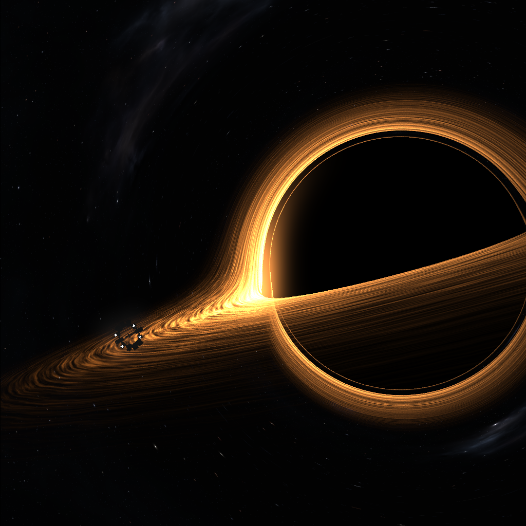
You can clearly see the gravitational lensing effect of the black hole, bending the light from the distant stars. And of course, the accretion disk is actually flat, but it is warped by the black hole’s gravity, making it look like a warped ring around the black hole, as made famous by Interstellar. Also the photon sphere, the thin ring of light around the black hole, is visible clearly. This is the path of light that is just barely able to escape the black hole’s gravity, and is bent around the black hole multiple times before escaping. I think that’s a great place to stop.
Conclusion
Phew! That was a long journey, but I hope you enjoyed it. We started with the simple problem of finding the shortest path between two points in a flat 2D plane, and ended up recreating the black hole from Interstellar! Along the way, we learned about the metric tensor, the Christoffel symbols, the geodesic equation, and numerical methods like RK4. We also saw how these concepts are used in general relativity to describe the curvature of spacetime around massive objects like black holes.
I hope your attention span hasn’t been fried by TikTok and reels and shorts and you actually managed to reach the end of this post. If you did, congratulations! Hope you are now eager to implement this yourself! Please do reach out to me if you have any questions, or if you want to share your implementation! I would love to see it.